Regression Trees Explained: The Most Intuitive Introduction

The field of machine learning is often framed around two dominant classes of models: neural networks (NNs) and tree-based methods. Early in my ML journey, I found it surprisingly easy to build an intuition for how neural nets work. You take a weighted sum of your inputs, pass it through a non-linear activation function, and repeat across layers. Simple enough — at least on the surface.

Decision trees, on the other hand, might sound like a naive or overly simplistic approach at first. But once you try building and training one from scratch, things quickly get more involved. And if you dive into regression trees, where the goal is to predict continuous values like temperature or price, any initial intuition you had tends to fly out the window.

In this tutorial, I'll walk you through what I believe is the most intuitive explanation of regression trees. When I first tried to truly understand how decision (and especially regression) trees work, I found a chapter in the Yandex ML textbook incredibly helpful — though unfortunately, it's only available in Russian. This article is inspired by the way they break down the concept.

As always all the code for this tutorial you can find on my  GitHub.

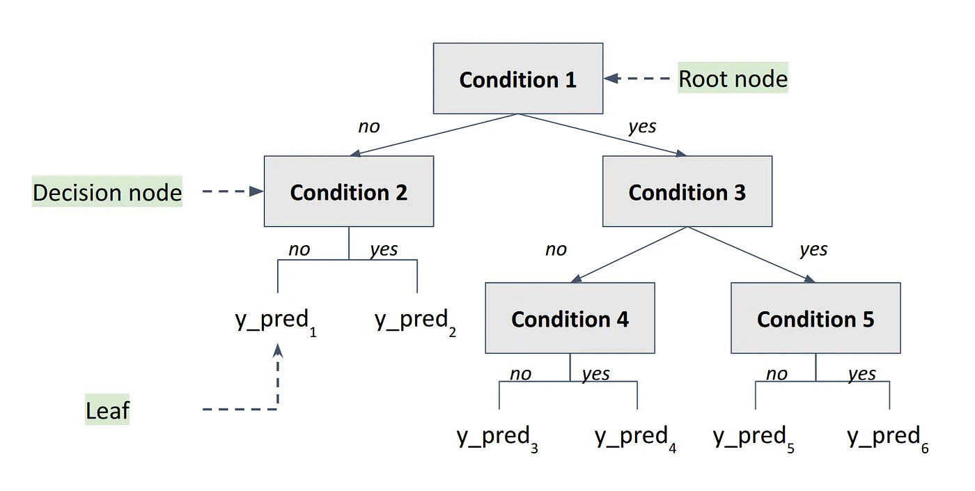
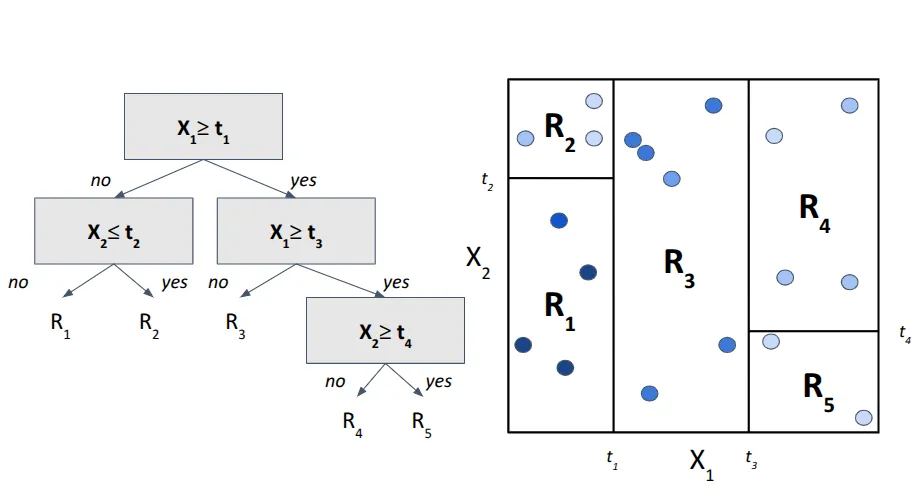
Let's begin by defining what a regression tree is. At its core, a tree is a graph-based model where each node represents a decision split (Fig. 1). These splits divide the data into regions in a way that optimizes a certain criterion. The key idea here is partitioning. So before jumping into the full algorithm, we'll go through a simple example to understand why this idea of partitioning is so important.

Intuition

Imagine that you are given a regression dataset with have two continuous features and one continuous target.

We can represent it as a 2D plot (Fig. 2), where the x and y axis represent X₁ and X₂, and the color of the objects represents their value of Y.

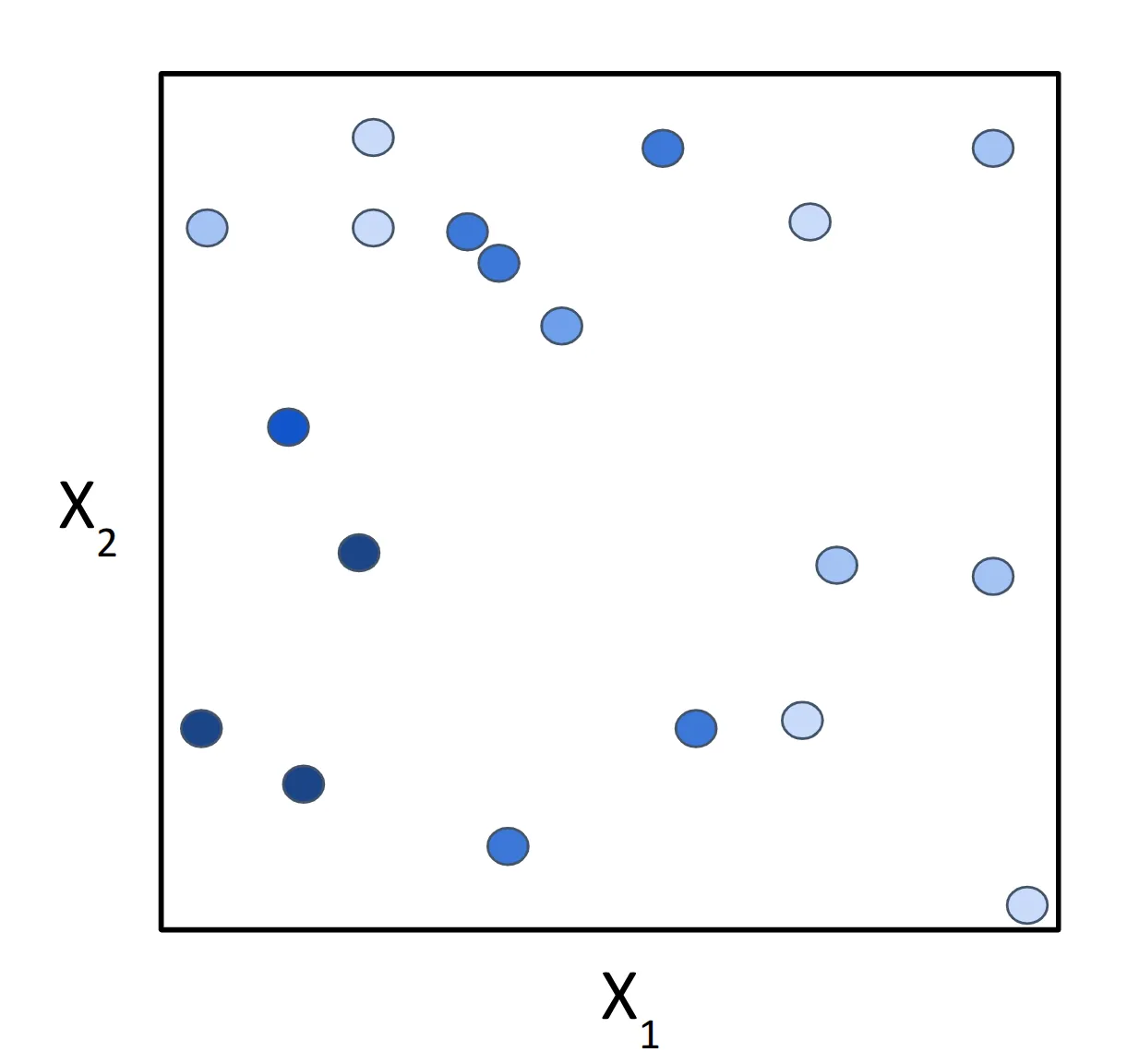
The goal of our decision tree is to split the feature space into a set of subspaces where the data points within each subspace are as similar to each other as possible. For now, we'll use arbitrary values for the decision nodes to illustrate the concept, but later, we'll dive into how these values are actually determined.

Step 1

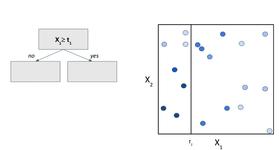
We start with a root node and define our first condition: if the value of feature X₁ is greater than some threshold t₁. Visually, this can be represented as a vertical line splitting the 2D space (Fig. 3). This split creates two subregions: left and right from t₁.

Step 2

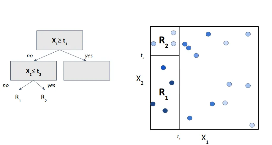
Now let's zoom into region left region. Within this subspace, we introduce a new condition — this time for feature X₂ with threshold t₂. The new split (a horizontal line) further divides the left region into two suspaces which we will call R ₁ and R ₂ (Fig. 4).

Step 3

By applying this process recursively (Fig. 5), i.e. splitting each region using simple threshold-based conditions , we keep dividing the space into smaller and more homogeneous subregions (resulting in R₁-R₅). The number of such splits is governed by the tree's depth, which corresponds to how many levels of decisions we make from root to leaf.

But now you might be wondering: “Okay, we split the space… so what?”

Well, here's the key insight — those regions define the model's predictions.

Each region contains training points with known values of the target variable Y. So when a new test point falls into one of those regions, the tree predicts its value as average of Y values from the training points in that same region (Fig. 6).

That's the core idea behind regression trees: instead of fitting a smooth curve, we're carving up the feature space into chunks where the target values are as homogeneous as possible. The tree learns to minimize variance within each region, making sure that the points grouped together are similar in value.

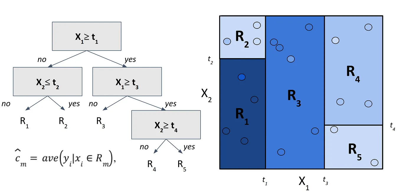
As you can see, the way regression trees make predictions is actually quite intuitive. We just split the space, group similar points together, and average their values. Simple, right?

But now we’re facing a few important questions:

• How do we choose the variable to split by, and where exactly to place the threshold?
• When should the tree stop growing?
• What are the limitations of this architecture? Can a tree really approximate complex, non-linear functions?

Let’s unpack each of these in the next sections.

Splitting

To answer the first question, let’s introduce the idea of information gain, a key concept in decision trees. In regression tasks, most of us in the machine learning world are familiar with Mean Squared Error (MSE). It’s the go-to metric for measuring how well our predictions match the actual values.

At each step in building a regression tree, the model asks a simple question: If we split the data at this point, will the overall MSE decrease? In other words, does dividing the data create a better, more informative structure , or are we better off stopping here and turning this node into a leaf?

So how does the tree decide where to split? There are several methods for finding a good threshold, but one of the most intuitive is based on percentiles of feature distributions. In a greedy, brute-force fashion, the tree goes through percentile values of each feature (in our case, just two), evaluating each one as a potential split point. If a threshold is found that reduces the MSE, the tree splits; if not, the node becomes a leaf.

Regularization

The second question brings us to an essential concept in machine learning: regularization. Without it, regression trees can easily overfit the training data, i.e. memorizing instead of generalizing.

To keep our tree in check, we introduce a set of parameters that control its growth and complexity:

• Maximum Tree Depth: Limits how deep the tree can go. Deeper trees can model more complex patterns but are more likely to overfit.
• Minimum Samples per Leaf: Specifies the minimum number of training samples required for a node to become a leaf. This prevents the tree from creating tiny, overly specific leaves.
• Minimum Samples per Split: Ensures that a node must have a certain number of training samples before it’s even considered for splitting.
• Minimum Information Gain: Sets a threshold for how much the MSE must decrease to justify a split. If the improvement is negligible (say, just 1e10−101) we skip the split to avoid unnecessary complexity.

…and there are other tuning knobs as well!

These hyperparameters act as guardrails, helping the model focus on meaningful patterns rather than noise.

Drawbacks?

Like any model, regression trees come with trade-offs.

• No extrapolation: Decision trees can't predict beyond the range of the training data. If you picture the feature space again, the tree makes predictions by partitioning it into known regions. So when it encounters an input that's far outside the range of what it's seen before, it simply can’t extrapolate a reasonable value.
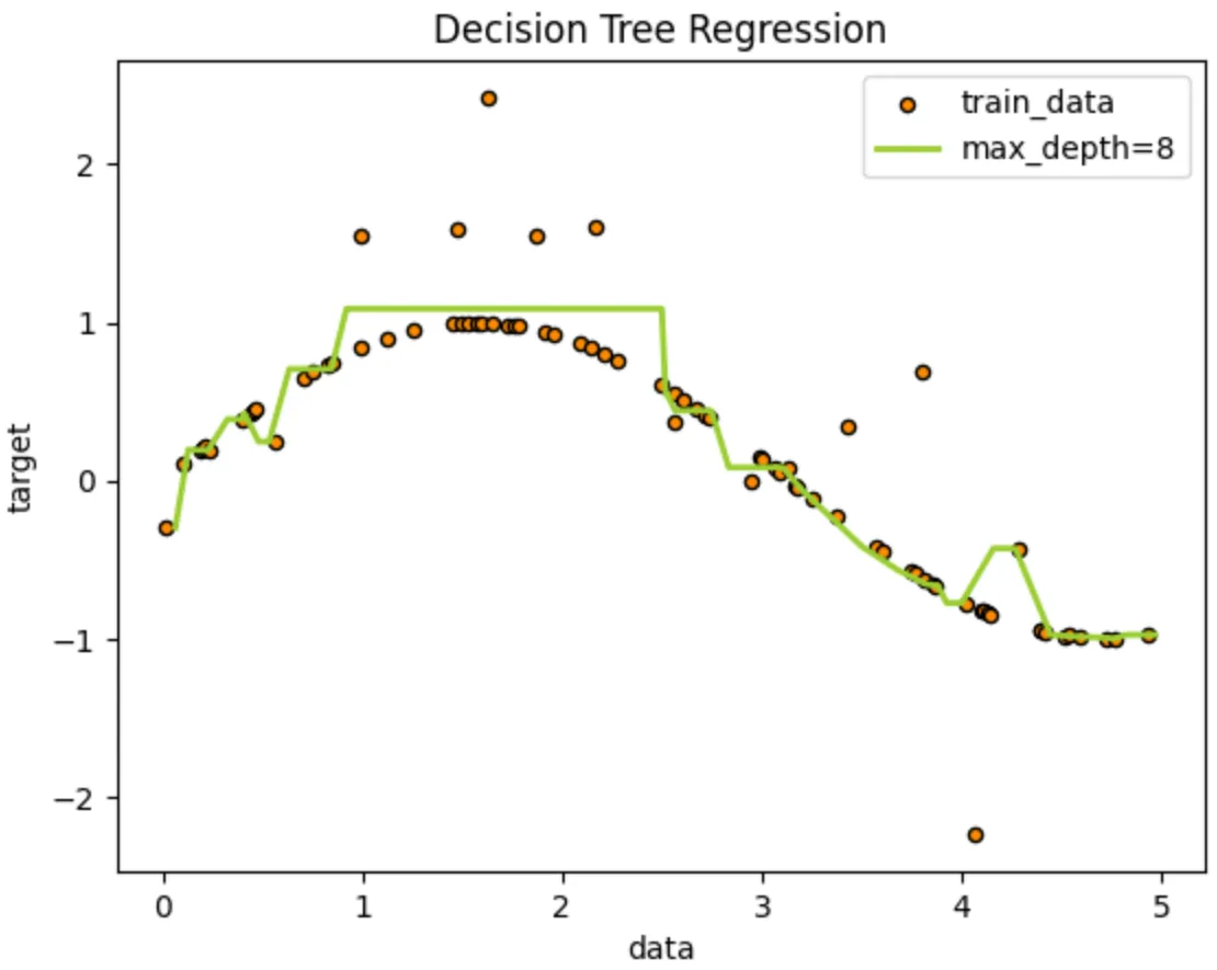
• Step-wise approximation: The output of a regression tree isn’t smooth — it looks more like a staircase (Fig. 7). That’s because the tree partitions the space into rectangular regions and assigns the average target value within each region. This step-wise prediction can be a poor fit for underlying continuous or smooth trends.
• Overfitting risk: Without regularization, a decision tree can easily overfit. In the worst case, it could memorize the training set (i.e. create one region per data point ) achieving zero loss on the training data, but performing terribly on new, unseen data.

---

Code

As is often the case in machine learning, implementing the model as a Python class is the most convenient and intuitive approach. We’ll start by defining two simple methods: the initializer and the criterion function. The __init__ method will store the structure of our tree, along with a regularization parameter, max_depth, to control how deep the tree can grow. The criterion method will be responsible for calculating MSE, which we’ll use to evaluate the quality of each split.

class RegressionTree:
  def __init__(self, max_depth=8):
    self.nodes = {}
    self.thresholds = {}
    self.leaves = {}
    self.max_depth = max_depth

  def criterion(self, true, pred):
    return np.linalg.norm(true-pred)

Next, let’s move on to the core part: training the tree. We’ll begin with the fit method. Its role is fairly straightforward: it takes the training data X and targets y, then calls an internal recursive method called grow_tree. Once the recursion is complete and the tree is fully built, we print a message just to confirm that the fitting is done.

def fit(self, X, y):
    self.grow_tree(X, y)

    print(f'Trained!')

Now, the heart of this model is the grow_tree method. This is where the actual recursion happens. The function continuously splits a parent node into two child nodes (left and right), creating new subspaces at each level. This process continues until a stopping criterion is met (like hitting the maximum depth or finding no useful way to split the data).

To keep track of the tree’s structure, we will use a simple but effective naming convention. Every node is assigned an ID, starting from root. Whenever we split left, we append _0, and for a right split, _1. So, a node with the ID root_0_0_1 means we went left twice and then right once (it’s quite a convenient pattern when visualizing or debugging your tree).

def grow_tree(self, X, y, depth=0, node_id='root'):
    X_l, y_l, X_r, y_r, depth, stop = self.split(X, y, depth, node_id)
    if not stop:
      for idx, data in enumerate([[X_l, y_l], [X_r, y_r]]):
        X_sub, y_sub = data
        child_id = f"{node_id}_{idx}"
        self.grow_tree(X_sub, y_sub, depth, child_id)

The main recursive logic lives inside the split function. It takes in:

• the current data (X, y)
• the current depth of the tree
• the node ID (for tracking the node’s position in the tree)

Within the function, we loop through each feature, and for each one, we generate a list of potential thresholds by computing 100 percentiles of its distribution. These thresholds act as candidates for splitting.

For each candidate threshold, the algorithm performs a virtual split of the data and computes the total error:

• First, we calculate the error before splitting — MSE of all y values at the current node.
• Then we compute the after-split error — the sum of MSEs in the left and right subsets.

If this split reduces the error (i.e. after-split error is smaller than the original), we store the corresponding threshold and feature index. After testing all possible thresholds, we proceed with the best one.

If no split improves the error (i.e. we’ve hit a stopping condition), we turn the node into a leaf. In this case, we simply store the mean value of y in that region and mark the node with a stop=True flag to end further partitioning. This is how recursion naturally halts when further splitting is not useful.

def split(self, X, y, depth, node_id):
  split_flag, best_feature_idx, best_threshold, best_criterion, stop = False, None, None, np.inf, False

  pred_no_split = [float(y.mean())]*len(y)
  no_split = self.criterion(y, pred_no_split)

  for feature_idx, feature in enumerate(X.T):
      thresholds = np.percentile(feature, np.arange(0, 101, 1))

      for threshold in thresholds:
        true_l, true_r = y[(feature<threshold)], y[~(feature<threshold)]
        pred_l, pred_r = np.mean(y[(feature<threshold)]), np.mean(y[~(feature<threshold)])
        split_l, split_r = self.criterion(true_l, pred_l), self.criterion(true_r, pred_r)

        split = split_l + split_r

        if no_split>split: #if error is lower when splitting
          split_flag = True
          if best_criterion > split: #if this split is better than all the previous
            best_feature_idx = feature_idx
            best_threshold = threshold
            best_criterion = split

  if split_flag == True and depth < self.max_depth:
    depth += 1
    self.nodes[node_id] = best_feature_idx
    self.thresholds[node_id] = float(best_threshold)

    y_l, y_r = y[~(X.T[best_feature_idx]<best_threshold)], y[(X.T[best_feature_idx]<best_threshold)]
    X_l, X_r = X[~(X.T[best_feature_idx]<best_threshold)], X[(X.T[best_feature_idx]<best_threshold)]
  else:
    self.leaves[node_id] = float(y.mean())
    stop = True
    y_l, y_r, X_l, X_r = None, None, None, None

  return X_l, y_l, X_r, y_r, depth, stop

Lastly, we need to implement the predict method so we can actually use our trained tree. The method works by iterating through each object in the test dataset and determining which leaf node it falls into by tracing a path from the root.

For every object, the traversal starts at the root node. At each node, the method checks whether the feature value is less than the current threshold. If it is, we move to the left child and append _0 to the node ID; otherwise, we move to the right and append _1. This process continues until we arrive at a node marked as a leaf, which we can recognize by the stop=True flag.

Once the leaf is reached, the method returns the stored prediction , or simply the mean of the target values from all training points that ended up in that region. Following this procedure for each object gives us a full set of predictions from our trained regression tree.

 def predict(self, X):
    preds = []
    for obj in X:
      node = 'root'
      while True:
        if node in self.leaves:
          pred = self.leaves[node]
          preds.append(pred)
          break

        feature = self.nodes[node]
        thr = self.thresholds[node]
        if obj[feature] > thr:
          node += '_0'
        else:
          node += '_1'
    return np.array(preds)

Testing

Now it’s time to put our regression tree to the test and see if it can actually solve a non-linear regression task. We’ll do this using two synthetic datasets, which give us full control over the underlying structure of the data.

Let’s begin with a simple case: a one-dimensional regression problem. We’ll generate a smooth curve (like a sine wave) and add some noise to simulate real-world data. The goal is to see whether the tree can approximate the non-linearity by learning meaningful splits and averaging the values within each partition.

rng = np.random.RandomState(10)
X = np.sort(5 * rng.rand(80, 1), axis=0)
y = np.sin(X).ravel()
y[::5] += 3 * (0.5 - rng.rand(16))

rng = np.random.RandomState(2)
X_test = np.sort(5 * rng.rand(80, 1), axis=0)
y_test = np.sin(X_test).ravel()
y_test[::5] += 3 * (0.5 - rng.rand(16))

Then let’s train two trees with different depths and get their predictions:

tree = RegressionTree(max_depth=4)
tree.fit(X,y)

tree2 = RegressionTree(max_depth=8)
tree2.fit(X,y)

y_1 = tree.predict(X_test)
y_2 = tree2.predict(X_test)

We will definitely need a code for visualization:

plt.figure()
plt.scatter(X, y, s=20, edgecolor="black", c="darkorange", label="train_data")
plt.scatter(X_test, y_test, s=10, edgecolor="black", c="black", label="test_data")
plt.plot(X_test, y_1, color="cornflowerblue", label="max_depth=4", linewidth=2)
plt.plot(X_test, y_2, color="yellowgreen", label="max_depth=8", linewidth=2)
plt.xlabel("data")
plt.ylabel("target")
plt.title("Decision Tree Regression")
plt.legend()
plt.show()

As you can see in Fig. 8, our regression tree does a solid job at approximating the non-linear function we created. When the tree depth is set to 8, it clearly overfits — capturing even small fluctuations caused by noise. In contrast, the tree with depth 4 produces a much smoother and more generalizable result.

For the second experiment, let’s explore how the regression tree partitions data in a two-dimensional space. To do that, we’ll generate a dataset with two input features:

n = 10000
x1 = np.random.uniform(0.01, 1, n)
x2 = np.random.uniform(0.01, 1, n)
X = np.column_stack([x1,x2])
y = np.where(
    (x1 < 0.8) & (x2 > 0.9),
    np.sin(1 / (x1 * x2 + 1e-3)),
    3 * np.exp(-(x1 - 0.5)**2 - (x2 - 0.5)**2)
)

n = 1000
x1_test = np.random.uniform(0.01, 1, n)
x2_test = np.random.uniform(0.01, 1, n)
X_test = np.column_stack([x1_test,x2_test])
y_test = np.where(
    (x1_test < 0.8) & (x2_test > 0.9),
    np.sin(1 / (x1_test * x2_test + 1e-3)),
    3 * np.exp(-(x1_test - 0.5)**2 - (x2_test - 0.5)**2)
)

Which will look like this (Fig. 9):

As a result, we can visualize each iteration of the tree-building process and compile them into a beautiful GIF:

---

Summary

In this tutorial, we tried to brake down regression trees from both intuitive and implementation perspectives. While decision trees may initially seem simplistic, building one from scratch reveals the smart mechanics behind recursive partitioning and variance reduction. By visualizing how the feature space is split and how predictions are made within regions, we demystified the way these models learn. With even a basic tree, we’ve seen how powerful this method can be in capturing non-linear relationships , especially when you’re in control of the algorithm’s logic. Whether you’re new to machine learning or looking to strengthen your fundamentals, understanding regression trees from the ground up is a rewarding step forward.